


1. INTRODUCTION
ShadowCam is a NASA Advanced Exploration Systems instrument hosted onboard the Korea Aerospace Research Institute (KARI) Korea Pathfinder Lunar Orbiter (KPLO), also known as Danuri. The design is based on the Lunar Reconnaissance Orbiter Camera (LROC) Narrow Angle Camera (NAC) but optimized for imaging of permanently shadowed regions (PSRs). PSRs never see direct sunlight and are illuminated by light reflected from nearby topographic facets (Watson et al. 1961; Shoemaker et al. 1994; Gläser et al. 2018).
This secondary illumination is very dim; thus ShadowCam was designed to be ≈200× more sensitive than the LROC NAC (Robinson et al. 2010). As a result, ShadowCam allows for unprecedented views into the shadows but saturates while imaging sunlit terrain.
ShadowCam provides critical information about the distribution and accessibility of water ice and other volatiles at exploration relevant spatial scales (1.7 m/pixel from 100 km altitude) required to mitigate risks and maximize the results of future surface activities. The ShadowCam investigation has five focused science and exploration objectives: 1. Map albedo patterns in PSRs and interpret their nature: ShadowCam will search for frost, ice, and lag deposits by mapping reflectance with resolution and signal-to-noise ratios comparable to LROC NAC images of illuminated terrain. 2. Investigate the origin of anomalous radar signatures associated with some polar craters: ShadowCam will determine whether high-purity ice or rocky deposits are present inside PSRs. 3. Document and interpret temporal changes of PSR albedo units: ShadowCam will search for seasonal changes in volatile abundance in PSRs by acquiring monthly observations. 4. Provide hazard and trafficability information within PSRs for future landed elements: ShadowCam will provide optimal terrain information necessary for polar exploration. 5. Map the morphology of PSRs to search for and characterize landforms that may be indicative of permafrost-like processes: ShadowCam will provide unprecedented images of PSR geomorphology at scales that enable detailed comparisons with terrain anywhere on the Moon.
Fig. 1 is a cutaway showing many of the key components of the ShadowCam instrument. Additional drawings and more detailed descriptions are in the ShadowCam instrument paper (Robinson et al. 2023). ShadowCam was designed and built by Malin Space Science Systems (MSSS). The design is inherited from the LROC NAC (Robinson et al. 2010) with several modifications to optimize for the challenging lighting within PSRs and accommodation on the KPLO spacecraft. These modifications include: 1) redesign of the focal plane, 2) increased baffling to reduce stray light, and 3) a new passive radiator design.
To provide increased sensitivity, the LROC detector was replaced by the Hamamatsu S10202-08-01 Time Delay Integration (TDI) Charge Coupled Device (CCD) and a new focal plane array (FPA) electronics board was designed and built by MSSS to support the new detector. This detector has 128 stages of TDI but for ShadowCam Hamamatsu installed a physical mask above the focal plane surface to block the illumination of some of them, giving effectively 32 stages of TDI. The TDI direction is commandable. We describe the two opposite directions as TDI A and TDI B. Six of the outputs of the detector are digitized in parallel to 12-bits and then companded to 8-bits. Each of these 6 channels handles a 512 photoactive pixel section of the detector, for a total format of 3,072 pixels. The detector is located next to the lightshield at the center of the focal plane electronics board, the first of four electronics boards shown in green in Fig. 1. A close-up of the focal plane electronics board is shown in Section 3.3.
For smaller PSRs, rejecting stray light is the biggest challenge for obtaining high quality images. Fig. 1 shows the vanes on the inside of the sunshade. The number of sunshade vanes was increased from six for the LROC NAC to twelve for ShadowCam, a secondary mirror inner baffle was added, two vanes were added to the primary mirror central baffle, the field flattener lens diameters were increased by 0.150 inch to reduce edge scattering, and a lower-reflectance surface finish was used on the light shield immediately above the detector. These modifications improved stray light rejection as shown in Section 7.1.
The radiating surface of the zenith-facing radiator will sometimes be exposed to the Sun, requiring that it have low solar absorptivity (α) while maximizing IR emissivity (ϵ). Optical solar reflector (OSR) material was used for this surface (α = 0.1, ϵ = 0.86), enabling the radiator to maintain the detector below 20°C even under the least favorable thermal conditions.
Table 1 gives a summary of ShadowCam performance and requirements where applicable. For parameters affected by TDI, the performance reflects the output signal after TDI. The modulation transfer function (MTF) is described in Section 2.2.
The table lists “shallow” and “deep” values for several parameters. The ShadowCam detector has 6 channels, each with 512 active columns. Channels 0–2, the shallow side, share an analog to digital converter (ADC) input, as do channels 3–5, the deep side. Early in calibration, after instrument integration, it was discovered that the 3 channels on the shallow side had much lower full well than the three channels on the deep side. The high signal striping and pepper noise described in Section 4.2 was also noticed. Eventually both effects were traced to a small discrepency in timing between the detector and the electronics. The engineering model electronics were updated and spare detectors showed much higher full well and no high signal striping and pepper noise. However, because the existing instrument met requirements and it was fairly late in the integration and delivery process, updating the flight electronics was deemed not worth the technical and schedule risk.
ShadowCam has commandable gain for each channel, with 64 levels that sample logarithmically over a gain range of about a factor of 5. The gain control parameter can have values from 0 to 63. Early in calibration gain parameter 35 was used in all the channels and the maximum signal was determined by the analog full well of the detector. For flight higher gain was used, with gain parameter 48 on the shallow side and 38 on the deep side. With the flight gains the maximum signal is determined by the maximum 12-bit value 4,095 DN of the output of the ADC. That’s the value given in Table 1. For both the shallow and deep sides of the detector, this value is only a little bit less than the analog full well, optimizing the digital sampling on each side while retaining almost the entire dynamic range. The gain is commandable in flight but we do not expect to change the gains. All DN levels quoted in this paper are 12-bit DN with the flight gain parameters of 48 on the shallow side and 38 on the deep side.
Table 1 lists 32 effective stages of TDI, but the Hamamatsu S10202-08-01 detector has 128 stages of TDI. The change from 128 to 32 was the result of a design decision early in the program.
The ShadowCam design phase included a thorough analysis of the signal to noise ratio (SNR) and dynamic range. Two models of the instrument were used, one based on modeling each component and one based on calibrated LROC performance with ShadowCam components substituted for LROC components. There was good a priori agreement between the two models, and later there was good ex post facto agreement with the ShadowCam instrument responsivity measured in laboratory calibration.
There was also a thorough analysis of typical radiance levels in PSRs based on long-exposure LROC NAC images. The analysis was performed separately for PSRs in the north and south polar regions.
For the nominal 100 km orbit, the instrument modeling and PSR radiance analyses indicated that a substantial percentage of pixels in the PSRs would be saturated, that is have signal larger than the top of the ShadowCam dynamic range. If the number of TDI stages were reduced to 32, very few PSR pixels would be saturated. There would be some loss of SNR in other pixels, but getting complete images of the PSRs was a higher priority. Note with 32 stages of TDI ShadowCam is still very sensitive. As shown in Table 1, SNR > 100 for radiance > 0.12 W/m2/sr/µm. On the dim side, in some cases ShadowCam is able to image the night side of the Moon using Earthshine (Wagner et al. 2023).
The number of TDI stages in the detector is not commandable but the vendor Hamamatsu had an option to ship the detectors with a physical mask installed above the focal plane. The mask nominally blocks detector rows 1–48 and 81–128, leaving rows 49–80 at the center of the detector illuminated, for a total of 32 illuminated TDI stages. The detector rows that are masked still contribute to the bias, dark current, and noise.
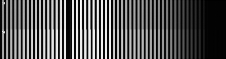
Also, since the mask is not located at the focus, the boundaries of the illumination are not perfectly sharp at the focal plane. Fig. 2 shows the illumination of the ShadowCam detector rows for a uniform target. This figure is a plot of the decompanded and bias subtracted DN in column 1,570 for lines 4,568–4,695 for image sfsh1_20210225_06_002. Pixel number 1 in the figure, corresponding to row 1 in the detector, is line 4,568 in the image. This image was taken with a Paul C Buff Inc Einstein E640 flashlamp uniformly illuminating a Labsphere Spectralon target. The flashlamp is on for a time much shorter than the line time. For a normal TDI image, the detector row signals at subsequent times get summed. But for this image, once each detector row gets illuminated, there’s no subsequent signal and the signal in a detector row just gets passed to the end of the TDI stages. Therefore the resulting image is just the image on the rows of the detector.
The mask is centered on the center of the detector rows. About 20 rows are fully illuminated and there are about 13 partly illuminated rows on each side, which appear to linearly fall off from the plateau. This would give equivalent TDI signal of approximately 20 + (13 / 2) + (13 / 2) = 33 or approximately 32 rows, as expected. About 41 rows on each side are unilluminated.
Table 1 gives the inverse gain and responsivity, which we can use to convert the detector noise and maximum signal to DN and then radiance, assuming a nominal 1.11 ms line time for a 100 km altitude orbit. That gives a dynamic range of 0.00036 to 0.55 W/m2/sr/µm on the shallow side and 0.00035 to 0.75 W/m2/sr/µm on the deep side for the nominal orbit.
The 12-bit raw DN values are companded to 8-bit values before downlink. To enable fast pixel readout, the companding table is a piecewise linear function. ShadowCam has flexibility to define and command different companding tables in flight subject to the piecewise linear limitation, where each linear piece has slope 2−M. M is an integer in the range 0–5 that can change from one linear piece to another but should always increase with signal. For convenience we limit ourselves to the 6 companding tables shown in Fig. 3.
Science images taken in lunar orbit almost all use the nominal companding table. The linear1 companding table (8-bit equals 12-bit for 0-255 DN) was used in laboratory calibration for darks and many low signal images, but it is not ideal because a single 8-bit value corresponds to widely separated 12-bit values. Darks taken in lunar orbit all use the painless linear1 companding table. This table has 8-bit equals 12-bit only up to 112 DN but each 8-bit value corresponds to just a local range of 12-bit values. This is true for all the companding tables except the linear1 table.
Decompanding is to the center of the range of 12-bit DN values consistent with the 8-bit companded value, except for for the linear1 companding table where the 12-bit decompanded value is set equal to the 8-bit value.
Images will be delivered to the NASA Planetary Data System (PDS) in environmental data record (EDR) and calibrated data record (CDR) format. These will not include any images in units of decompanded 12-bit DN. EDRs are companded 8-bit DN and CDRs are calibrated radiance in W/m2/sr/µm. The calibration pipeline converts the EDR to the CDR. The first step is decompanding the EDR to 12-bit DN.
The ShadowCam calibration pipeline may be expressed by the following Eq. (1).
Each of the 6 channels for each TDI direction has its own set of parameters. The subscript i denotes the channels, k is the TDI direction (A or B), x is the column number within each channel, and y is the image line number. Lical (x,y) is the best estimate from the data of the true scene spectral radiance Li(x,y). It is weighted average spectral radiance of the scene pixel over the ShadowCam bandpass. The weighting function is the spectral responsivity rik(λ), which is related to the radiometric calibration coefficient Rik as described in Section 6.
The TDI direction k is commanded to A or B depending on which way the spacecraft is flying. The relative A/D converter gain is gi. It is defined to be 1 for the standard flight gain for each channel, which is commanded as gain parameter 48 for channels 0, 1, and 2 and 38 for channels 3, 4, and 5. The gain parameter can run from 0 to 63 and the gain is approximately logarithmic with gain parameter. The signal for gain parameter 63 is approximately 5 times the signal for gain parameter 0.
The line time is τ. That’s the time from the start of the exposure in one line to the start of the next line. The effect of the TDI multiplier on exposure time is accounted for in Rik.
Ni(x,y) is the count in each pixel after decompanding, in other words the 12-bit DN.
Pi is the median of the bias pixels for all bias pixel columns and all lines in the given channel in that image. Line-by-line subtraction of the bias was tried but it is not used because it introduced horizontal striping.
T is the detector temperature. Two temperatures measured on the detector board are reported. Sensor A is attached to the heat sink line that connects the detector mount and the radiator, and it was determined to be much better correlated with dark signal, so we use that value. The variation in detector temperature within a single image is small and a single temperature value is used for each image.
Section 3 describes the derivation of the tables for dark signal subtraction. For a set of dark images with multiple line times at a single temperature T from laboratory thermal vacuum testing, the signal Ni(x,y) for the given TDI direction k as a function of line time τ was fit column-by-column to the linear function Mik(x,T) + τDik(x,T). The slope and intercept were calculated from dark images with line times covering the range 0.3–2.0 ms. This procedure was repeated for a set of different temperatures T. The derived linear fit coefficients were then fit column-by-column to an exponential function of T. This fit resulted in the dark signal calibration tables Qik(x), Kik(x), Cik(x), and Jik(x). These tables are used in the calibration pipeline as shown in Eq. (1) to subtract dark signal. Qik(x)eKik(x)T is the model of the intercept of the dark signal Mik(x,T) and Cik(x)eJik(x)T is the model of the slope of the dark signal Dik(x,T).
Fik(x) is the flat field image calibration table, the image of a uniform radiance scene at relatively low count levels (Ni(x,y) ≈ 700 shallow side, ≈ 500 deep side) where the high-signal striping artifacts described in Section 4.2 are not present. As described in Section 4.1, the flat field tables are calculated from laboratory data using an illuminated Spectralon panel as the uniform source. Each table is normalized to have a mean of 1 within the channel, so channel-to-channel variations are accounted for in the radiance calibration coefficient Rik.
Rik is the radiance calibration coefficient. It converts counts to spectral radiance in W/m2/sr/µm and accounts for variations in response between the channels and between the TDI directions. The derivation of Rik is described in detail in Section 6.
2. IMAGING PERFORMANCE
Focusing is critically important to meeting the MTF requirement of ≥ 0.2 at Nyquist that flows from the exploration and science requirements of the ShadowCam program.
The ShadowCam telescope is a Ritchey-type Cassegrain with the secondary mirror located by a composite tube and internal spider structure (Robinson et al. 2010). The composite structure was chosen for its combination of strength and low mass but the material is hygroscopic and increases in length as it absorbs water.
The instrument has no provision for in-flight focus compensation, and the design goal is to keep the focus fixed under flight conditions by using a composite with a low coefficient of thermal expansion (CTE) and keeping the tube dry. The tube is initially dried out during cruise to eliminate CTE effects on focus.
The goal of ground focusing of ShadowCam before launch was to set the flight fixed focus as close to infinity as possible. Setting focus was complicated because the tube is completely dry in flight (after the cruise bakeout operation) but it is not completely dry in the lab at ambient pressure, temperature, and minimum humidity required for electrostatic discharge (ESD) protection.
Focus of the telescope before electronics integration was by autocollimation - repeated measurements were taken as the structure was baked out and the tube was judged to be dry when the focus position stopped moving.
The optics focus testing above verified that there is no astigmatism - the correct detector position is the same for best downtrack and best crosstrack focus. It also provided a predicted location along the optic axis to place the Shadowcam detector for best focus.
In order to place the detector in the focal plane assembly (FPA) at the correct position along the optical axis, the design incorporates a focus position shim. Instrument focus was tested with different thicknesses of shim installed, using an external collimator with optics identical to Shadowcam.
Instead of a pinhole or typical resolution target, the target at the focus of the collimator was a transparent flat plate with a series of bars in a repeating pattern with a spatial period of 666 microns, as shown in Fig. 4. The plate was tilted at an angle of 2.23° with respect to the focal plane of the collimator so that it was focused at infinity only at one location of the bar pattern. That location was determined using autocollimation with a large optical flat. It was identified subsequently by counting bars from a single wider bar in the pattern as shown in Fig. 4.
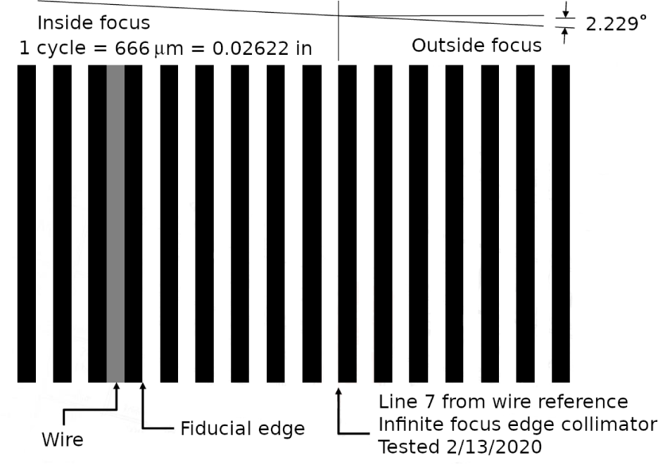
With the focus shim, flight FPA, and flight detector in place on the flight instrument, the shim thickness was evaluated and updated by measuring cross-track focus. The boresight of the collimator was aligned with the ShadowCam boresight and the collimator was oriented so that the bars of the tilted plate target extended downtrack. The crosstrack position in the bar pattern of best focus of the resulting ShadowCam images was compared to the location of infinity focus of the collimator as previously determined by autocollimation.
An initial focus evaluation was performed on the benchtop using the collimator and bar target but the shim was not updated.
The steps of the process to update the shim were as follows. ShadowCam was baked out in a thermal vacuum chamber for the time and temperature previously determined to make the tube dry and the focus stable at the flight value. The temperatures were then set near those expected on orbit. The collimator was viewed through a window in the vacuum chamber. Images of the collimator target were acquired and custom software was used to determine the MTF at 1/12 Nyquist spatial frequency for each edge in the bar target. The peak MTF was compared with the position of the tilt target infinity focus. If they differed, we fabricated a new focus shim with thickness calculated so peak MTF would be at the tilt target infinity focus. Then we broke vacuum, disassembled ShadowCam to provide access to the FPA and focus shim, and installed the new shim.
We repeated the process described in the previous paragraph until the peak MTF measured in the ShadowCam images was at the tilt target infinity focus. The shim was updated 3 times before correct focus was verified.
Imaging performance is verified by measuring the MTF. We used the same bar target as used for focusing, tilted with respect to the focal plane. The measurement was done at ambient during benchtop calibration. Because the instrument was not at its dry focus, we calculated MTF from the sharpest dark-to-light transition in the image, rather than using the tilt target infinity focus location. This MTF measurement was therefore not a verification of focus. It is correct only if the focus determination described in the previous section is correct.
Often MTF is measured with an edge slightly slanted with respect to the the columns of the image, in order to achieve sub-pixel sampling of the line spread function. To do this with a pushbroom TDI camera such as ShadowCam would require scanning the camera. Our intent was to measure MTF from many images with the best focus edge in different positions, but given the combinations of companding table and signal level, only a few of the bar target images turned out to be appropriate for MTF measurement. We ended up calculating MTF based on one laboratory calibration image scmt0_20210514_03_009 and did subpixel sampling by linear interpolation.
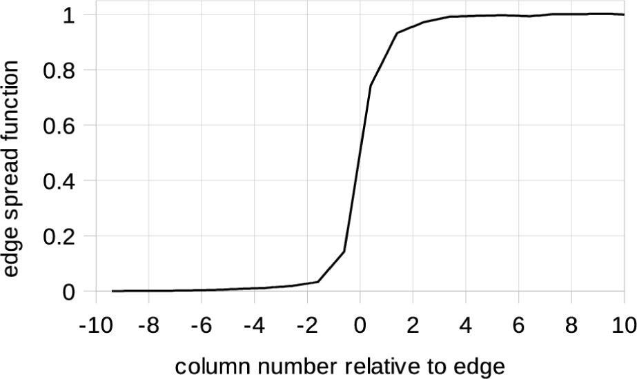
We then calculated the edge spread function (ESF). We averaged all rows of the image and used 20 columns close to the sharpest dark to bright transition. Fig. 5 shows that function, normalized so the bright side is 1 and with the x-axis translated to put x = 0 at the edge.
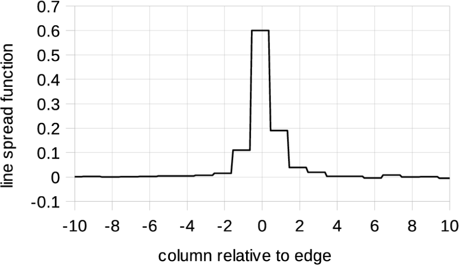
The line spread function (LSF), shown in Fig. 6, gives the image of a vertical bright line of infinitesimal width on a dark background. It is just the derivative of the ESF. The blocky appearance is a consequence of using just one image to calculate the ESF and using linear interpolation for subpixel sampling of the ESF.
The MTF, shown in Fig. 7, is just the modulus of the Fourier transform of the LSF, normalized to equal 1 at zero spatial frequency (Hecht 1987). The value estimated from this laboratory image is 0.21 at the Nyquist spatial frequency of 0.5 cycles per pixel. This meets the requirement of MTF > 0.2 at Nyquist, which means the optical performance takes full advantage of the pixel scale. It is very similar to the MTF of the LROC NAC (Humm et al. 2016), which has the same optics.
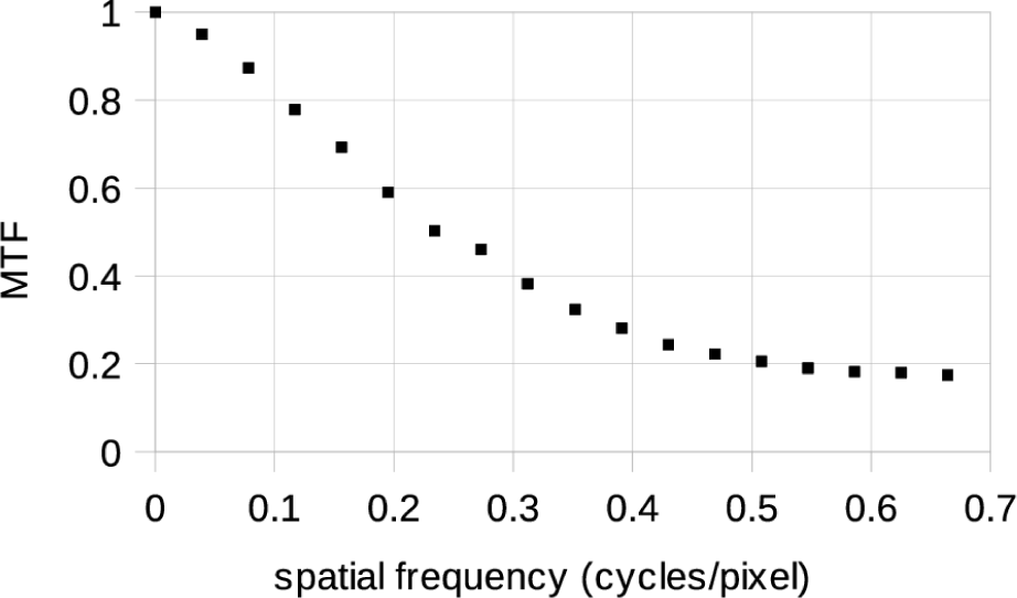
With the same optics one would expect the same MTF for ShadowCam and the LROC NAC at the same spatial frequency measured in cycles per µrad. However, ShadowCam has 17 µrad sampling versus 10 µrad for the LROC NAC. The larger pixel sampling means the Nyquist frequency in detector-independent units is 0.029 cyc/µrad for ShadowCam versus 0.05 cyc/µrad for the LROC NAC. As shown in Fig. 7, MTF is higher at lower spatial frequency, so the ShadowCam MTF would be expected to be higher at Nyquist. There are two effects that lower the measured ShadowCam MTF down to about the level of the LROC NAC.
The first is a measurement effect. The ShadowCam MTF is measured with a target image that includes aberrations from the collimator which are similar to those of the ShadowCam telescope itself. The LROC NAC MTF was measured in flight from the limb of the Moon against dark space, which is a good approximation of a perfect light to dark edge. So it seems likely the true MTF of ShadowCam is higher than the LROC NAC. This higher MTF would apply to images of the Moon taken in flight.
The second is a detector performance effect. ShadowCam has a column transfer signal artifact, discussed in the next section. This reduces the MTF. The LROC NAC also has such an effect but it is corrected in signal processing of the final image (Humm et al. 2016). It may be possible to improve the performance of ShadowCam with an analogous correction.
One essential function of the ShadowCam FPA electronics board is to provide a clocking signal to smoothly pass electrons down the CCD through the 128 TDI stages and then across the detector through the serial buffer to the analog-to-digital (A2D) converter located at the corner of each channel. However, the timing of this clock is slightly offset, causing a portion of the electrons passing through the serial buffer to lag. This is most noticeable after abrupt changes in signal level (especially high signal to low signal). Fig. 8 is a comparison of two images with the same target. This is the tilted bar target described in the previous two sections. Both images are calibrated except for the last step of radiometric calibration, conversion of DN to radiance. Note that these images were taken with lower gain, gain parameter 35, than the flight gains of 48 on the shallow side and 38 on the deep side. Since the calibration includes a gain correction to the equivalent DN using the higher flight gains, it is possible for the calibrated DN to be higher than the 12-bit limit of 4,095. The same is true for Fig. 9. Calibrated DN levels higher than 4,095 indicate signal near analog signal saturation, since the flight gains were chosen to be close to the analog signal saturation levels.
The images in Fig. 8 are displayed conjoined for comparison of the width of the bars. The top image a, scmt0_20210514_02_017, has a short line time of 0.32 ms for lower signal level and the bottom image b, scmt0_ 20210514_02_007, has a long line time of 4.10 ms for higher signal level. They are stretched differently in Fig. 8 so the brightness of the bars is similar despite the great difference in signal level. In the ideal case, the shape of the bar target is the same in all images; the only change should be an increase in the signal and dark current.
Fig. 8 shows two characteristics of the effect of the charge transfer lag on images. In the center of the field, where the bars are brightest, the higher signal bars at the bottom are wider in the image than the lower signal bars at the top. The increase in width is at the right edge of each bar. At the left and right ends of the field, where the bars are dimmer, the higher signal bars at the bottom don’t appear any wider than the lower signal bars at the top. Note also the widening effect is stronger on the shallow side (the left half) of the detector than the deep side (the right half).
Fig. 9 shows profiles of a single bright bar of the tilted bar target in images with different line times to give different signal levels. These are calibrated (again, without the final step converting DN to radiance) images from image set scmt0_20210514_02 and the plot is approximately centered at column 1,274. As the signal level increases, the sharpness of the dark-to-light transitions decreases, and a rounded shoulder appears in the profile at the left edge of the bright bar. The rounded shoulder does appear to diminish for the highest signal profile but that is for a signal level close to analog saturation.
The charge transfer lag also causes the right edge of the bright bar to move to the right, when the signal goes from light to dark in Fig. 9. In this orientation, the serial buffer moves the signal from the right side of the detector to the A2D converter on the left side of each channel. While this lag effect does not drastically change the qualitative interpretation of the ShadowCam images, it makes the images less sharp, quantified by lower MTF. It elongates bright areas above or near instrument saturation into adjacent dimmer regions of the image.
The profiles in Fig. 9 also show a four-column pattern. At high signal level the DN decreases systematically every four columns. This is the high signal striping effect discussed in Section 4.2.
Because it is due to the signal lag, the column signal transfer effect occurs within each line of the image independently. It is primarily an artifact that reduces image sharpness, but it also has an effect on images of a uniform target. These create an additional image artifact but also help characterize the effect quantitatively which may help to implement a correction in the future.
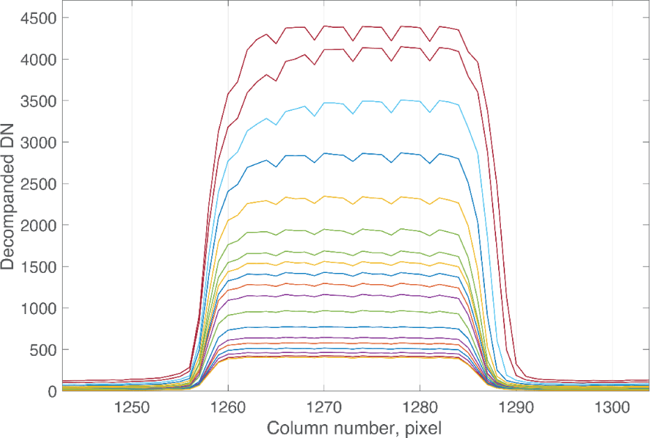
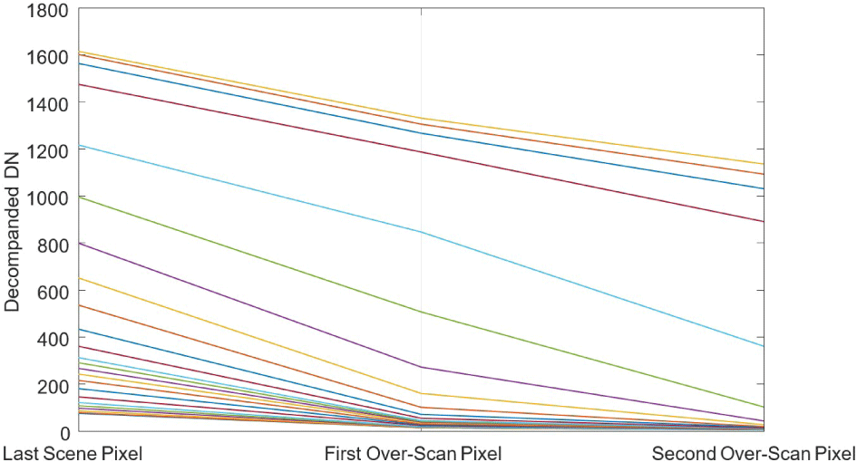
The structure of ShadowCam uncalibrated (EDR) images is discussed in detail in Section 3.1. For each channel the instrument records two “virtual” pre-scan pixels, eight bias pixels, the 512 scene pixels, and two “virtual” over-scan pixels during the readout of each row. The “virtual” pixels are not present on the detector but are generated by clocking the A2D two times before and after reading the physical pixels on the sensor. The eight bias pixels are physically located on the detector but they are not light sensitive. They are used to carry charge away from the photo-sensitive portion of the CCD to the A2D converter.
Under normal circumstances, the 12 pixels not associated with the scene pixels should read out the bias signal level of the channel. However, the two over-scan pixels in bright scenes contain residual charge due to the signal lag, as shown in Fig. 10. Furthermore, the first scene pixel (left-most on the detector) does not reach its actual value since some of its charge is passed to the pixel to the right. The amount of charge shifted to the right is non-linear, as shown in Fig. 11, further complicating the characterization and eventual corrective actions. For example, to first order the flat field calibration step corrects the reduced signal level of the first column in each channel, but only at the signal level used for the laboratory flat field measurements. Often a dark vertical stripe is observed at the first column of a channel in a calibrated image due to increased charge transfer in brighter regions of the image, not fully corrected by the flat field calibration step.
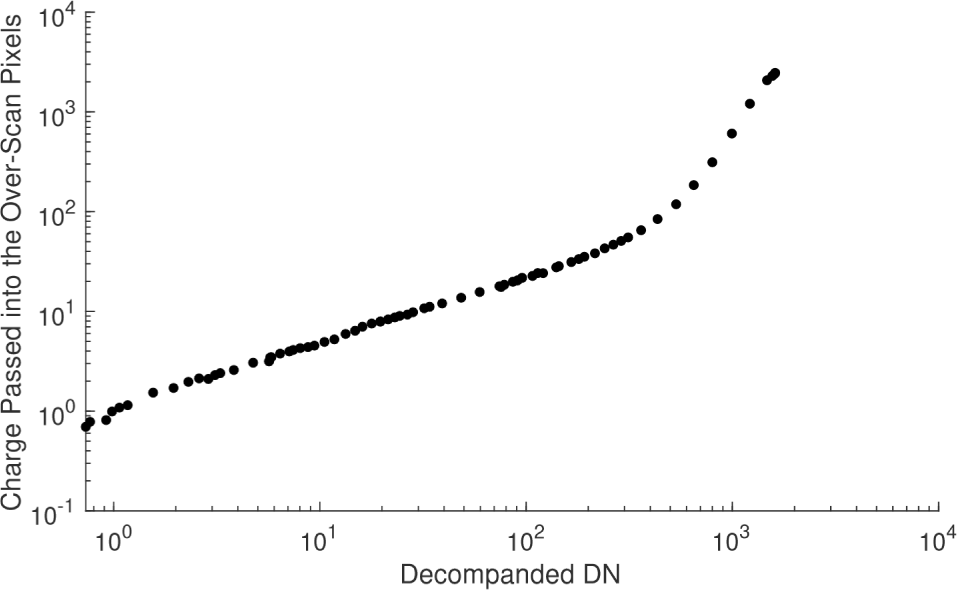
Figs. 10 and 11 are based on laboratory images of a uniform target. Many such images are available covering the range of signal levels. In theory it is possible to analyze the overscan pixels and the first column of each channel, model the nonlinear function shown in Fig. 11, and correct the images by subtracting the modeled transferred signal, a nonlinear function of the signal in the previous one or two columns in the current line. As of this writing, the correction has not been implemented.
3. DARK SUBTRACTION
Each channel of the detector is separated by unresponsive columns (“bias pixels”) which are easily identifiable in a raw image except for a short exposure or cold temperature dark image. Because each of the six channels has a different analog signal chain, including for each TDI direction, we calibrated each channel independently, essentially resulting in the separate calibration of 12 channels.
Fig. 12 is a schematic of the structure of the uncalibrated (EDR) images. Each line of pixels in a given channel is comprised of 2 “virtual” pre-scan pixels, 8 bias pixels, 512 scene pixels, and 2 “virtual” overscan pixels, as described in the previous section. Only the scene pixels are included in the final calibrated image, which has six channels with 512 pixels each, resulting in an image that is 3,072 pixels across.
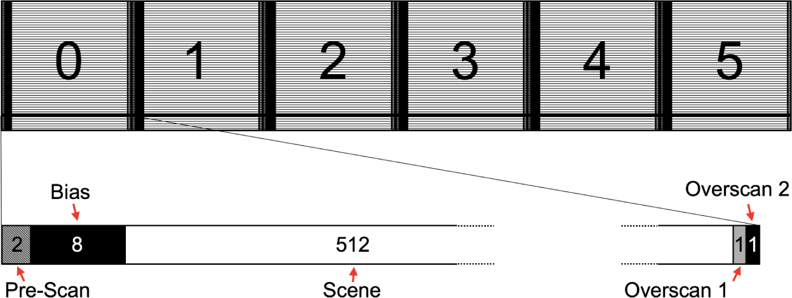
The bias pixels do not respond either to light or to thermally induced dark current. These pixels were used to monitor the zero signal DN level in each image. Initially, a line-by-line bias pixel subtraction was attempted, where the mean of the eight pre-scene bias pixels in each line was subtracted from each scene pixel in that same line. However, this introduced unwanted horizontal image striping. Instead, for the final calibration, the mean of the block of eight bias pixels for all lines in the image was subtracted from each scene pixel in the image.
Fig. 13 shows linearity plots at the low end of the dynamic range for dimly illuminated images at room temperature and for dark images at +33°C. The signal levels are similar. At room temperature the signal from images sptf1_20210512_07_001 through 024 is dominated by the illumination, but also the dark signal is subtracted using dark images sptf1 20210512_05_001 through 024 with the same line times. The darks at +33°C were images tvdarkramp157_20210618 through tvdarkramp180_20200618 from thermal vacuum testing, bias pixel subtracted and corrected for a temperature drift between the images. The order of the start times of the dark images was different than the order of the line times of the images, and the images were multiplied by a factor linearly dependent on the start time to compensate for a temperature decrease linear with start time. The correction was optimized for a monotonic and smooth increase in signal with line time, and the time-dependent factors were all between 0.9 and 1.1. The channels with higher response in all the images are of course the shallow channels which use larger gain.
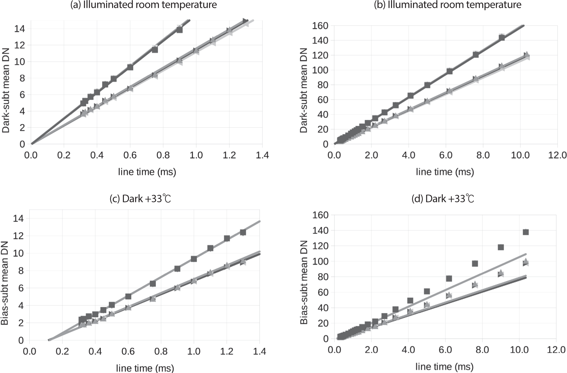
The plots on the right show the full commandable range of line times 0.3–10.35 ms, and the plots on the left are close-ups for short line times to show the behavior at the lowest signal levels. All the plots include a linear fit to the subset of shorter line times 0.3–2 ms.
The response to photons is very close to an ideal linear response while the dark current is slightly nonlinear. Not only does the dark current response curve upward at higher signal, but the intercept of the fit to the 0.3–2 ms line time data is –1 DN versus 0 DN for the illuminated case.
If one compares dark images with different temperatures and therefore different dark current levels by scaling line times to match the bias-subtracted DN, the curves fall on top of each other. This indicates the nonlinearity in the dark current depends only on signal level.
A linear function with a nonzero intercept is a good enough approximation to the dark current for line times 0.3–2 ms and detector temperatures –20°C to +35°C, which covers all flight cases. Therefore we modeled the dark current with a linear function for simplicity. Both the slope and intercept depend on detector temperature and that is discussed in the next section.
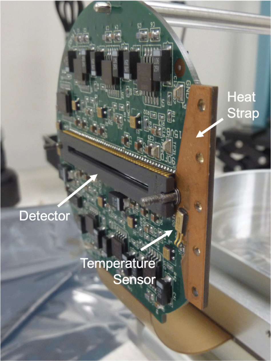
Laboratory dark image tests were conducted in instrument level thermal vacuum testing over the temperature range –30°C to +50°C, larger than the design requirement of –20°C to +35°C and much larger than the observed range in lunar orbit of –10°C to +10°C. The detector reads out temperature at two locations on the instrument, one on each side of the detector. The temperature measured at the interface of the heat strap and the detector, detector temperature A, was determined empirically to be much better correlated with dark signal so that temperature was used in the modeling and for applying the model to calibrate flight images. Fig. 14 shows the detector, the heat strap, and the sensor for detector temperature A.
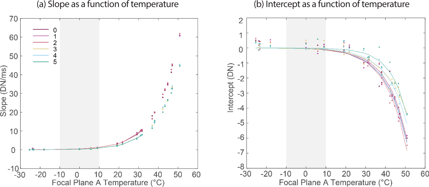
At each temperature the line time was varied over the course of the test. The dark current model was derived by first a linear fit of bias-subtracted dark signal as a function of line time at each temperature to give slope and intercept at each temperature, and then an exponential fit of slope to temperature and an exponential fit of intercept to temperature.
First a linear regression was fit to the median DN value of the scene pixels in each column of each channel (512 total) as a function of line time τ for the set of images at each temperature T. The median value in each column was used since it is less sensitive to outliers compared to the mean. The linear function was restricted to line times of 0.3–2 ms due to the nonlinearity of the detector response at low signal levels as described in the previous section. The linear fit resulted in values of the slope Dik(x,T) and the intercept Mik(x,T).
An exponential function was then fit to each term (slope and intercept) of the column-by-column linear fit as a function of temperature (Fig. 15). So Qik(x)eKik(x)T is the model of the intercept of the dark current Mik(x,T) and Cik(x)eJik(x)T is the model of the slope of the dark current Dik(x,T). For TDI B, the exponential fit for slope was restricted just to the design requirement operating range (–20°C to 35°C). However, for TDI A, due to a gap in valid laboratory data between –18°C to 0°C (see Fig. 15), a larger range of –30°C to 35°C was used for the slope fit, extending beyond the low end of the operating range to ensure a good fit. The exponential function for the intercept was fit to the full temperature range –30°C to +50°C of laboratory data for both TDI directions.
In the calibration pipeline, the fitted exponential functions are evaluated at the detector temperature of the flight image to give slope and intercept. Then the linear function is evaluated at the line time of the flight image to give modeled dark signal which is subtracted, column-by-column, from the bias-subtracted image as described in Eq. (1) and Section 1.2.4 above.
At the time of laboratory calibration and dark current analysis, the in-flight instrument performance and thermal prediction was unknown. Therefore, it was critical to quantify the detector behavior over a wide range of temperatures. Due to good thermal performance the range of ShadowCam temperatures is much smaller in flight, and almost all the dark corrections are less than 3 DN.
4. IMAGE UNIFORMITY
Bias and dark current are additive artifacts in the raw image. Once those are subtracted, the next calibration step is to divide out spatial nonuniformity of response. The flat field calibration table is just a normalized image of a uniform source. Since ShadowCam is a pushbroom type imager there is no downtrack dependence so the flat field calibration table Fik(x) is just one dimensional with 3,072 values, one for each column. There are two tables for the two TDI directions. Images of a uniform target were calibrated through dark subtraction and then the column means were taken. They were then normalized within each channel to give a nominal flat field table for each image. These tables were averaged and processed as described below to give the table Fik(x) used in the calibration pipeline.
Fig. 16 shows the configuration for the flat field, photon transfer, linearity, and radiometric calibrations. A Gamma Scientific Spectral LED RS-7-1 with a 3-inch diameter port illuminates a 24 × 24 inch Labsphere SRS-99 Spectralon panel oriented for normal illumination, and the ShadowCam instrument observes from an angle.
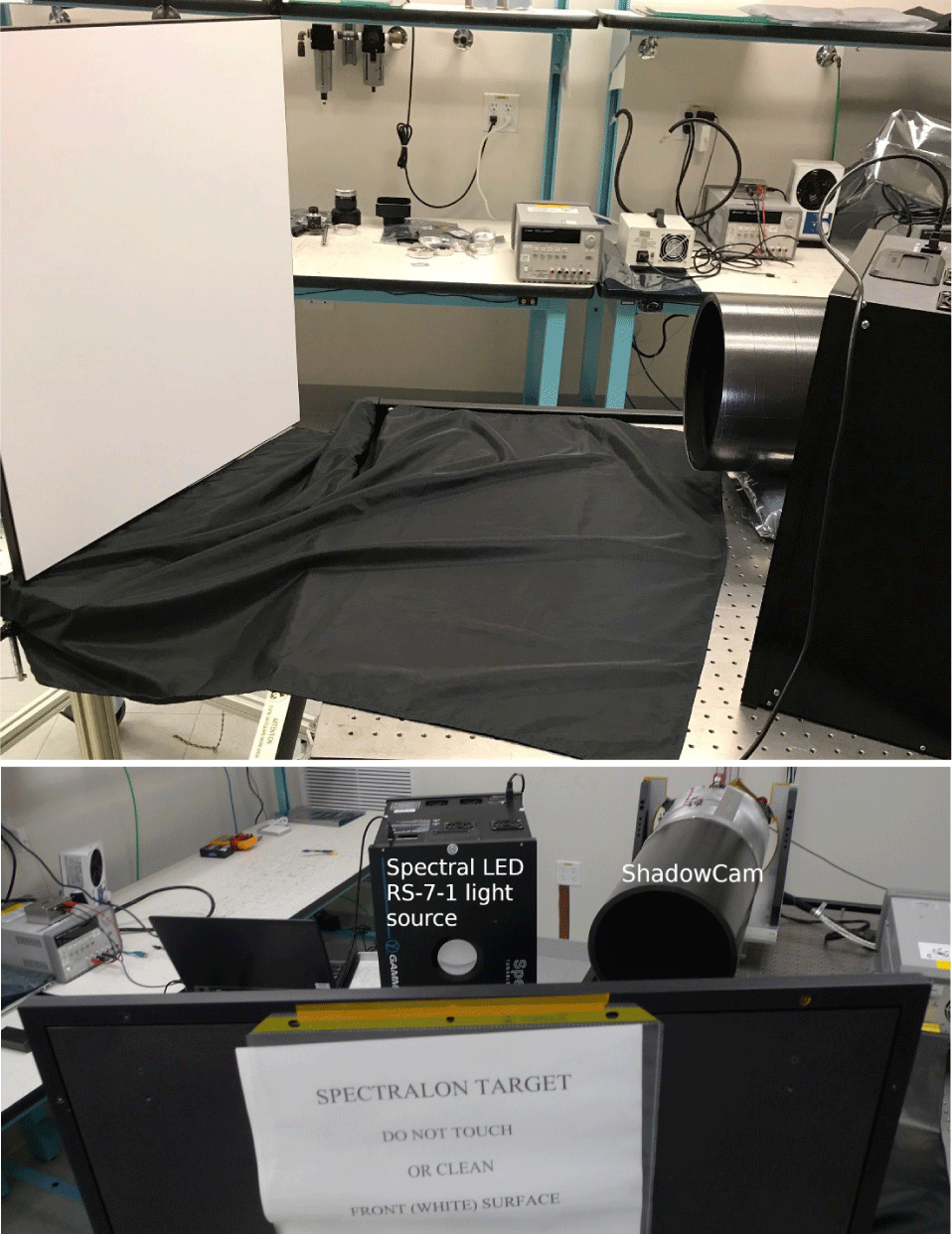
The Spectral LED RS-7-1 light source uses 32 independently commandable LEDs for illumination, each with a different wavelength. The 28 used for the ShadowCam calibration have centroid wavelengths in the range 394–807 nm and each was used separately for illumination of an image for the radiometric calibration, as discussed in Section 6.1. For the flat field images, the LEDs were used simultaneously to approximate a given spectral radiance function. A function was chosen proportional to the solar spectral radiance times the square of a nominal lunar reflectivity function linearly increasing from 400 nm to 800 nm, in order to approximate the spectral radiance of a PSR with secondary illumination.
The illumination and line time were chosen to give enough signal for good SNR but not to get into the regime of high-signal striping and pepper noise as described in the next section. Converting from the non-flight gains used for the laboratory flat field images to flight gains, the signal levels were 600–775 DN for the shallow side and 440–570 DN for the deep side.
In the top image in Fig. 16, the panel is illuminated from the left as seen from ShadowCam. This was the configuration for TDI A images sptf0_20210302_04_009, sptf0_20210302_04_018, sptf0_20210302_04_022. The bottom image in Fig. 16, on the other hand, shows the panel illuminated from the right as seen from ShadowCam. This was the case for TDI A imagesffd0_20210303_04_002 and TDI Bimages sptf0_20210511_04_009, sptf0_20210511_04_ 018, and sptf0_20210511_04_022. These images in these two configurations were the full set of laboratory images used to make the flat field calibration table Fik(x). This geometry gives the best target uniformity for side illumination of a flat diffuse panel. The small remaining nonuniformity has a side-to-side component and a radial component.
The side-to-side component, due to slightly higher reflectance at a smaller backscattering angle (the panel is not perfectly Lambertian), was measured by a comparison of left and right illuminated images. The mean of the 3 TDI A flat field images with left illumination was calculated and the average of that mean with the single TDI A left illuminated flat field image was calculated. The ratio showed a change of 0.69% over the entire ShadowCam field of view (FOV) for left illuminated versus the average of left and right. The change is approximately linear with field angle. This result agrees with laboratory measurements of the slight angular nonuniformity of the target using a light meter centered at the ShadowCam aperture. For TDI A the production flat field table was calculated from the average of left and right illuminated flat field tables. For TDI B we used only images with right illumination. A correction was applied to the radiometric calibration coefficients Rik of the 6 channels for TDI B to account for the side-to-side nonuniformity. No correction was applied to the flat field table Fik, which is normalized within each channel (see Section 1.4.4), leaving a systematic radiometric error in each TDI B channel with maximum value ± 0.06% in the first and last columns. This is too small to lead to any significant image artifacts but is included in the flat field error budget.
The radial component is due to several effects. The center of the illumination pattern is the closest point on the panel to the source. It’s also is the only point with zero incidence angle at the panel and zero emission angle at the port of the source. Using the inverse square law and the cosines of the incidence and emission angle these effects were estimated to give a target brightness dropoff of < 0.1%, < 0.05%, and < 0.05% respectively from the center to the edge of the ShadowCam FOV. The resulting total is < 0.2%. This is small so it was just folded into the uncertainty and no correction was made for the radial nonuniformity of the target.
Figs. 17 and 18 show the ShadowCam flat field calibration table Fik(x) for the shallow side and the deep side of the detector respectively. The different channels i are shown as different plots, and the different TDI directions k are plotted on top of each other. As expected the TDI A and TDI B flat fields track each other very closely for slow changes over the focal plane.
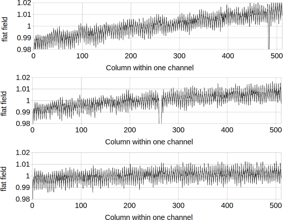
As discussed in Section 1.4.4, the flat field calibration table Fik(x) is normalized to 1 within each channel, and the channel-to-channel instrument response variations are accounted for by the radiance calibration coefficient Rik. One can see from the shapes of the plots in Figs. 17 and 18 that the instrument response falls off toward the edges of the field of view. The values of Rik obtained from the radiometric setup were adjusted to reflect the channel-to-channel variations obtained from the flat field setup, which was optimized for target uniformity. The final values for the relative response for the different channels were 1.134, 1.158, 1.170, 0.855, 0.850, and 0.833 for channels 0–5 respectively for TDI A and 1.138, 1.156, 1.166, 0.857, 0.850, and 0.832 for TDI B. As expected, one sees good agreement between TDI A and B, the gain difference between shallow and deep, and a drop-off toward the edge of the field of view.
There is a 4-column pattern which is considerably larger on the shallow side of the detector than the deep side. Fig. 19 gives a close-up of the first 100 columns of the shallow channel 2 and the deep channel 3 to illustrate this more closely. The 4 column pattern is not perfectly repeating, and there are small differences between TDI A and TDI B.
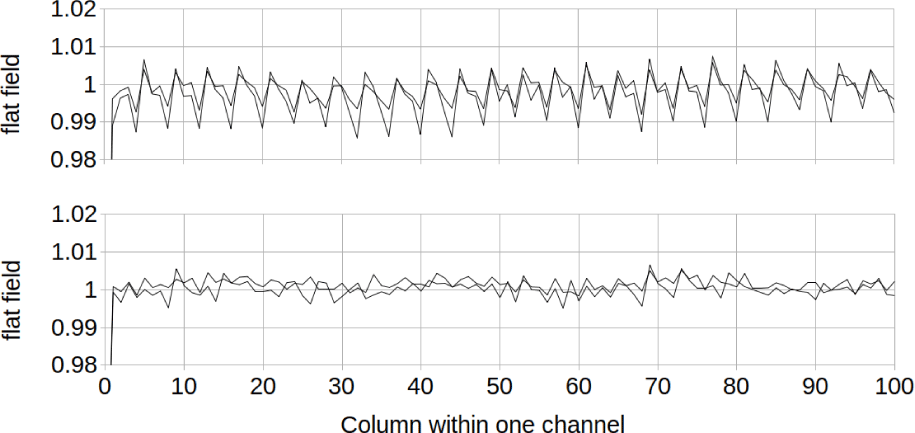
The uncertainty in the 4-column pattern was estimated to be 0.1% from a similar close-up plot from all 6 channels with a flat field calculated from each separate image. The detail seen in Fig. 19 repeats very well in the flat fields calculated from the individual images after each column is averaged. Random noise in the laboratory flat field images does not significantly contribute to the uncertainty because the images were averaged over 1,024 lines for use in the flat field tables.
To calculate the total uncertainty we add in quadrature the contribution of 0.2% from radial nonuniformity of the target, 0.06% from side-to-side nonuniformity within each channel, and 0.1% nonrepeatability in the 4-column pattern. The result is 0.23% uncertainty in image spatial uniformity. This includes the uncertainty at high spatial frequency within each channel accounted for by the flat field calibration table Fik(x) and at low spatial frequency accounted for by the radiometric calibration coefficients Rik. This uncertainty is much smaller than the SNR and so doesn’t contribute to any significant image artifacts.
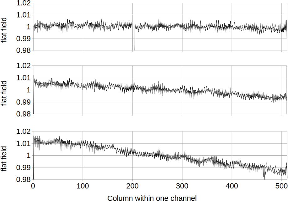
There are a few large artifacts visible in Figs. 17, 18, and 19, with low values below the lowest range of the plot. In Fig. 19 the first column in each channel is low. This is a result of the column transfer of signal discussed in Section 2.3. For the first column in each channel, the signal is transferred from the bias pixels instead of an illuminated pixel resulting in a lower total DN. The resulting values in the flat field table are 0.808, 0.831, 0.819, 0.921, 0.903, and 0.915 for the first column of TDI A channels 0–5 respectively, and 0.822, 0.871, 0.859, 0.932, 0.952, and 0.954 for TDI B.
Some other dips below the range of the plots are evident in Figs. 17 and 18. These were not present in the laboratory calibration images, but were introduced after the first images were taken from lunar orbit. Dark vertical stripes were observed in many flight images. We believe they are due to particles settling on the detector between laboratory calibration and lunar orbit, perhaps during launch. The particles may be black paint from the detector housing which was optimized to have very low and diffuse reflectivity in order to minimize stray light. An empirical correction was made to the laboratory derived flat field table, using lines 10,276–12,775 of lunar image M013428232S, a relatively uniform area of a flight image. This correction changed columns 483-484 of channel 0, 260–265 of channel 1, and 200–204 of channel 3 in the flat field table. The lines of the calibrated image were averaged and the ratio of the affected columns to nearby columns was used to make the correction. The smallest flat field values in each of the corrected features is 0.934, 0.948, and 0.934 respectively. Since this is to correct an effect that removed signal, the flat field tables in the affected channels were not renormalized. This means no change was needed in the channel responsivity coefficients. The 3 dark vertical stripes disappeared from the flight images once the revised flat field was put in production.
Because the column transfer effect still leads to dark stripes in the images, and the accuracy of the correction for the 3 flat field artifacts was only confirmed by inspection of nonuniform flight lunar images, we choose to claim 1% spatial response uniformity in Table 1, rather than the value of 0.23% derived from the accuracy of the laboratory calibration. These values are for calibrated images, of course. It is also possible that we missed much smaller artifacts that appeared after laboratory calibration, but that seems unlikely. The 3 features observed all have the same depth, suggesting any additional features would have the same depth and therefore be evident in flight lunar images as vertical dark stripes. The 0.23% value for uncertainty in response uniformity is likely to apply to all of the image columns except the first column in each channel and the corrected columns.
The ShadowCam detector has excellent linearity and response uniformity at low signal levels, but at higher signals nonuniformity artifacts appear. Figs. 20 and 21 show a small area in 5 images of a uniform target. Fig. 20 is from the shallow side of the detector and Fig. 21 from the deep side, and the line time is different for the 5 different images for each. Each image is displayed stretched to approximately ± 5% from the mean in the patch.
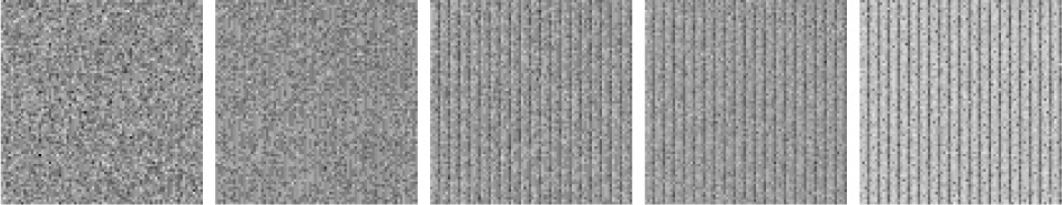
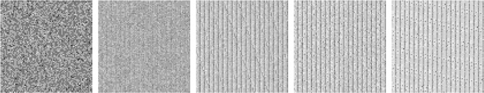
One can see two effects. The first is the normal random shot noise which decreases as the signal increases as expected. The second are patterns of pixels darker than the rest. These appear and become more prominent as the signal gets larger. There is a repeating pattern of a single column every 4 columns, the “striping”, and a varying but not random pattern of separated pixels, the “pepper noise”. These two effects have the same amplitude at the same signal level, an amplitude that reaches a maximum of approximately 3% at the largest signal levels.
One can see from the figures and captions that on the shallow side the effects are not significant up to about 860 DN and are very evident at 1,190 DN. On the deep side they are not significant up to about 1,300 DN and very evident at 1,910 DN. The gain on the shallow side is about 1.3× the gain on the deep side, so the target radiance can be more than twice as big on the deep side before these artifacts appear.
Some work was done on a striping correction based on signal level. A correction based on one set of uniformly illuminated images was successful in removing the striping from another set, but the particular correction function chosen introduced striping at low signal level. So the correction is feasible but a function must be used that does not change the low signal images. The pepper noise does not have a fixed pattern so removing it would require a filtering algorithm that would be optimized to the amplitude and character of the pepper noise to minimize effects on small features in the images. Neither the striping correction or the pepper noise filtering are implemented in the calibration pipeline as of this writing.
5. GAIN, LINEARITY, AND SIGNAL-TO-NOISE RATIO
The photon transfer function shows the standard deviation in the signal, or its square the variance, as a function of the signal level. We can use it to determine the conversion between signal in a single pixel measured in DN and measured in electrons.
The photon transfer function was measured by uniformly illuminating a Spectralon panel with a Gamma Scientific Spectral LED RS-7 light source. This provided a target with spatially uniform and temporally stable radiance.
Let n be the signal in a single TDI-summed detector element in electrons and N = g n be the signal in DN, where (1/g) is the inverse gain in electrons/DN. Let σn and σN = gσn be the associated standard deviations. Take the standard deviation over a single column of the image. All the DN values in that column come from the same TDI-summed detector element. Because the light source is stable all the variation is from statistical noise. Then
where σshot is the shot noise and σread is the read noise (or zero point noise) measured in DN or electrons respectively. Then use n = (1/g) N and square both sides.
This equation predicts that σN2, the variance of DN, is a linear function of N, the signal in DN. The slope of that function is the gain and the intercept is the square of the gain times the square of the read noise in electrons.
Fig. 22 shows the column variance in DN as a function of the column mean DN, specifically the mean of each over all the columns of each channel. The DN values have bias pixel subtracton applied but no other calibration.
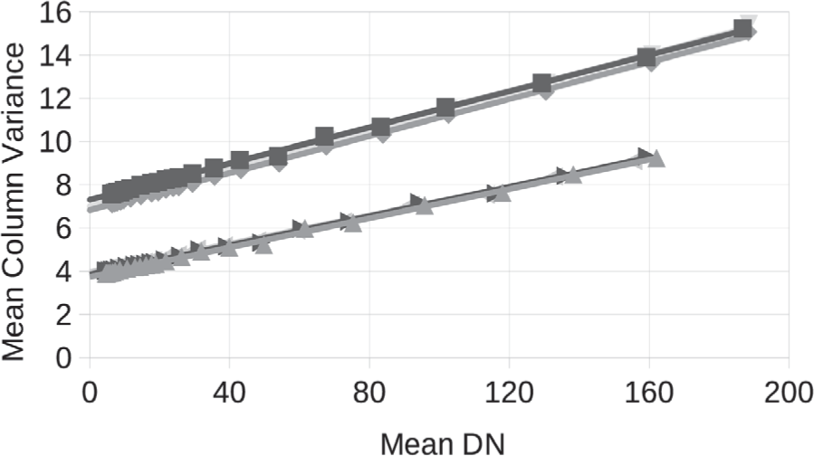
The data set consists of images sptf1_20210512_07_001 through 024 and used a companding table with 8-bit DN equal to 12-bit DN to avoid any changes in quantization noise with signal level. To use this companding table signal levels were chosen so all pixels of all the uncalibrated images had signal levels DN < 255. This also avoided the high signal pepper noise discussed in Section 4.2.
The behavior shown in Fig. 22 is close to the theoretical prediction, indicating good linearity at low signal level with no unexpected noise terms. For channels 0–2 which use higher gain the mean inverse gain is 23 e−/DN and the read noise 62e−. For channels 3–5 which use lower gain the mean inverse gain is 30 e−/DN and the read noise 58e−.
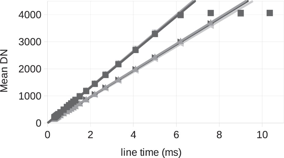
The photon transfer function indicates good linearity at low signal, but we can also look directly at dark subtracted signal as a function of line time to confirm linearity. Fig. 13(a) and 13 (b) show very linear behavior in the response to photons at low signal levels. Note the linear fit is to only the images with line times 0.3-2 ms but the line is a good fit all the way up to 10.35 ms.
Fig. 23 is a plot of the bias-subtracted mean signal in each channel for the images sptf0_20210512_09_001 through 024. Here also I include a linear fit to line times 0.3–2 ms and it fits the data well until the signal gets close to the maximum signal level of 4,095 12-bit DN. These plots confirm good linearity performance for both low signal and high signal.
We can plot the SNR for the whole dynamic range using the Fig. 23 dataset and calculating the standard deviation of each column. Fig. 24 shows the mean of these column standard deviations for each channel. The column standard deviation includes random noise such as read noise and shot noise. It would include any line-to-line variations, but for ShadowCam we have not noticed significant horizontal striping. Of the nonrandom effects discussed in Section 4.2, the pepper noise is included and the vertical striping is not.
SNR is defined as the ratio of signal to standard deviation. If we take signal N and divide it by the square root of Eq. (3) we get as a function of signal is expected to follow the formula . For small N, this formula is proportional to N and for large N to the square root of N. In any case it would increase monotonically as N increases.
Clearly Fig. 24 does not follow this theoretical behavior. At about DN = 500 there is a jog downward. This is due to increased digitization noise for DN ≥ 544, which the 8-bit companded image samples in steps of 16 DN, versus steps of 8 DN for DN < 544. Because this image set uses the entire dynamic range, it uses the default flight companding table 0 which approximates a square root function with a piecewise linear function. At higher signal level there is another companding table transition at a signal level of 2,208 DN, with steps of 32 DN above that level. Also the pepper noise described in Section 4.2 reduces the SNR at high signal levels.
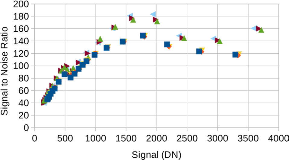
Fig. 24 does show good SNR performance over a wide range of signal levels. The three channels with higher SNR are the deep channels 3–5 and the three with lower SNR the shallow channels 0–2. This plot is a bit misleading because the shallow channels use higher gain so at the same DN they have a lower signal level than the deep channels. A fairer comparison is Fig. 25. This is the same plot but with the x-axis converted from DN to radiance, assuming the nominal 1.11 ms line time for a 100 km altitude orbit.
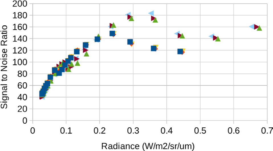
From the Figs. 24 and 25, SNR > 100 for signal > 790 DN or radiance > 0.106 W/m2/sr/µm on the shallow side and signal > 670 DN or radiance > 0.122 W/m2/sr/µm on the deep side. Both these levels suffer from the companding table transition at 544 DN, though. Below that transition the SNR stays high to lower levels than one might expect. SNR > 80 for signal > 450 DN or radiance > 0.060 W/m2/sr/µm on the shallow side and signal > 400 DN or radiance > 0.073 W/m2/sr/µm on the deep side.
6. ABSOLUTE RADIOMETRIC CALIBRATION
The spectral response was determined by illuminating a Spectralon panel with a Gamma Scientific Spectral LED RS-7-1 light source as was done for the photon transfer function, linearity, and flat field measurements, but taking one observation with each of 28 wavelengths of LED in the light source, from 394 nm to 807 nm.
The radiometric calibration of ShadowCam is ultimately derived from the National Institute of Standards and Technology (NIST) traceable calibration of the Spectral LED source, but ShadowCam observes the Spectralon panel illuminated by the source, not the source directly. To convert Spectral LED radiance to ShadowCam radiance, both were measured with a Thorlabs PM100D light meter across the entire wavelength range used for calibration. This was done with the light source, panel, and ShadowCam in their final positions for taking calibration data, with the light meter placed in the aperture of the light source and at the front of the ShadowCam baffle. The light meter used an adjustable iris with 9.5 mm diameter 90 mm from the 9.7 × 9.7 mm square detector surface, which made it sensitive to an approximately 5 × 5 inch patch of the panel, versus an 8-inch diameter circular patch for a single pixel of ShadowCam. The ratio of Spectralon to Spectral LED radiance is plotted in Fig. 26(b). This ratio accounts for the reflectance of the Spectralon panel as well as the distance of the Spectral LED illumination source.
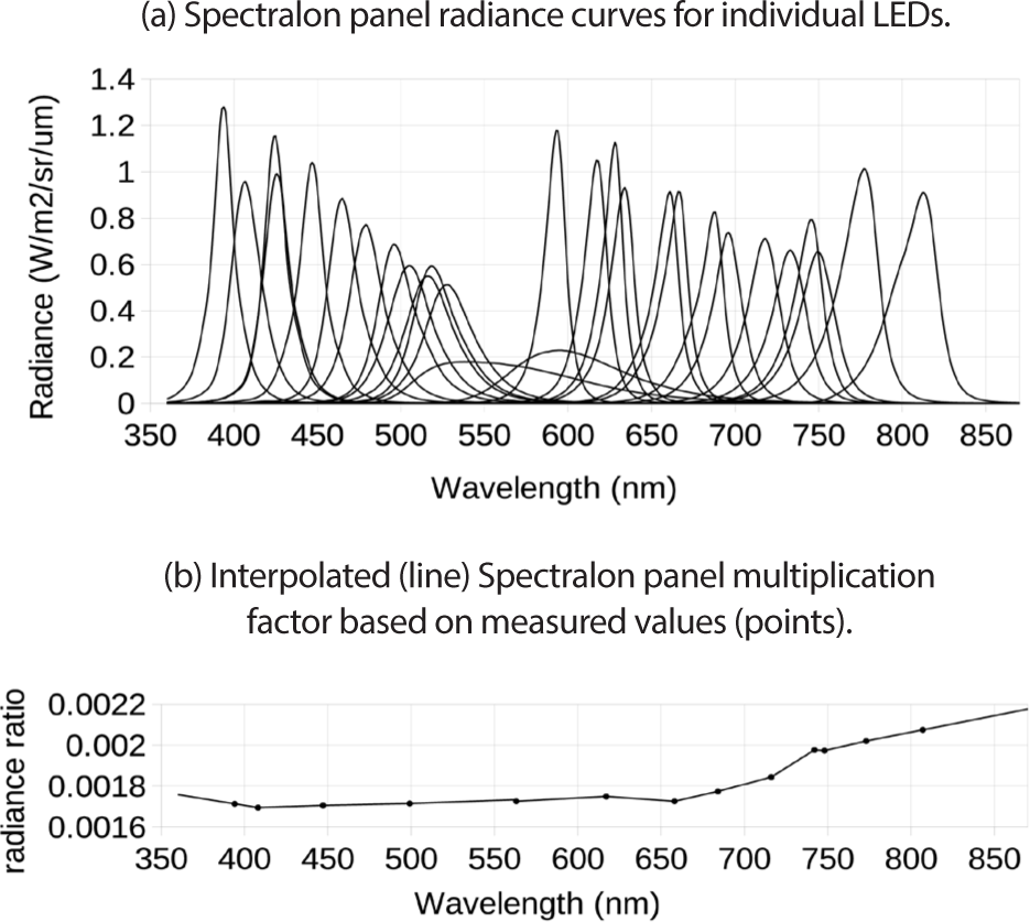
Using the geometry of the laboratory set-up one may calculate the radiance ratio for an ideal panel with 100% reflectance and Lambertian photometric function, and this gives an approximate check on the measured radiance ratio. The result is 0.00204. The values plotted in Fig. 26(b) range from 83% to 102% of that value, showing the measurement is in the right range. The spec for a pristine sample of SRS-99 Spectralon shows 98% reflectance at 400 nm and 99% over most of the bandpass. The lower values for this panel are not surprising given its age and use, and deviation of Spectralon from a perfect Lambertian photometric function could also have an effect.
The light meter had its own independent radiometric calibration of amps per watt of optical power as a function of wavelength. With the geometry of the iris it measured radiance in W/m2/sr, and we compared the radiance of the panel directly measured by the light meter versus that calculated from the Spectral LED radiance, with the light meter used only to convert source radiance to panel radiance. The directly measured radiance ranged from 7% lower at 395 nm to 11% lower at 656 nm to 3% higher at 805 nm, with an apparent systematic wavelength dependence. The range is a little surprising, but again the conclusion is that the Spectralon radiance calculated from the Spectral LED radiance is reasonable. Thorlabs quoted a 3% calibration uncertainty for the light meter but its calibration is not considered as rigorous as the Gamma Scientific calibration of the Spectral LED. Error could also arise in the Thorlabs radiance measurement from our use of the iris. The iris was adjustable so its diameter was measured by a precision calipers, and an error of only 0.1 mm would give a 2% radiance error. This uncertainty would not affect the conversion from source radiance to panel radiance because the iris was not adjusted between the measurements.
Each image used a single LED in the spectral light source. Fig. 26(a) shows the spectral radiance function of the Spectralon panel in units of W/m2/sr/µm for each LED. Most had relatively narrow wavelength bands (the majority of the signal falls within a few tens of nm of the peak), however two LEDs (nominally at 520 nm and 620 nm) had much wider response curves. These were used anyway as the spectral response curve was expected to be linear in that range, and few narrower-band LEDs covered the range. The light source output radiance for each observation was modeled at 1-nm intervals by the light source controller based on factory-provided LED response data. The wavelength value used for each LED is the centroid of that reported spectrum convolved with the Spectralon to Spectral LED radiance ratio, also linearly interpolated to 1 nm intervals as shown in Fig. 26(b). The reflectivity curve only changed the centroid of the broad-spectrum 604 nm LED, which had a pre-reflectance centroid of 605 nm.
We collected mean dark-corrected decompanded DN for each channel of each image in the test suite (28 wavelength bands ranging from 394–807 nm, one for each TDI direction, for a total of 56 images; srad8_20210513_02_001-056). For dark correction, we took the mean decompanded DN of each channel for dark images taken before and after the spectral image sequence at the same exposure times and TDI directions as the radiance calibration images (sdrk1_20210513_01_006, 01_021, 02_006, 02_021, 03 006, 03_021, 04_006, and 04_021; calibration images included two exposure times: the edges of the spectral range used longer exposure times than the middle). These before and after mean DNs were averaged to get a dark correction value for each channel/exposure/TDI direction combination.
For each dark-corrected image, we divided the mean DN for each channel by the line time to get instrument response in DN/ms. The recorded spectra were modified by the Spectralon panel reflectivity function, and integrated to get total reflected radiance in W/m2/sr. Finally, for each channel, wavelength, and TDI direction, we divided the reflected radiance by the instrument response to get the spectral responsivity Rik(λ) in (DN/ms)/(W/m2/sr) (see Fig. 27).
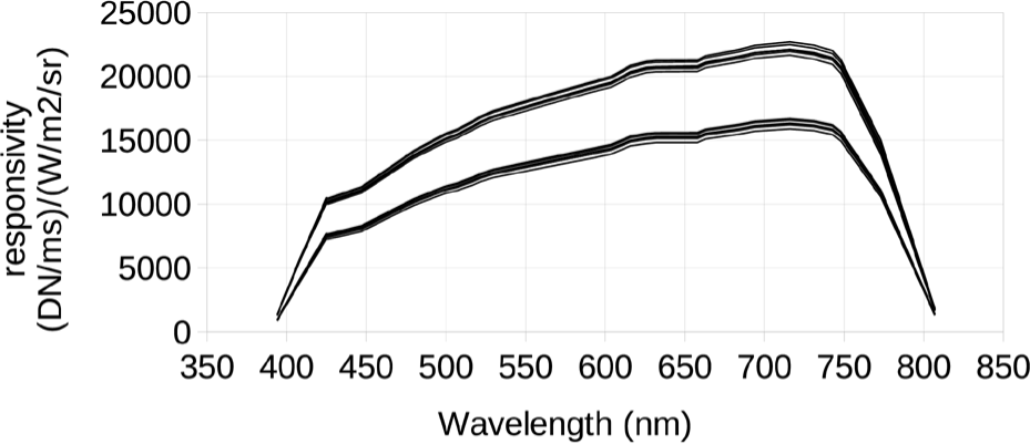
The spectral responsivity Rik(λ) gives the response of the instrument to monochromatic light with a given radiance, in units of W/m2/sr, and at a given wavelength λ. For the calibration pipeline we want the radiance calibration coefficient Rik, the integral of Rik(λ) over λ. Rik gives the response of the instrument to broadband light with a given spectral radiance in units of W/m2/sr/µm, constant across the bandpass of the instrument. When Rik is applied in the calibration pipeline, the result is an estimate of the weighted mean spectral radiance of the scene pixel, with the weighting function being the spectral responsivity Rik(λ).
For each TDI direction, we averaged the spectral responsivity values for the shallow (channels 0–2) and deep (channels 3–5) sides of the detector separately, then integrated under the averaged spectral responsivity curve, treating the curve as a series of linear line segments connecting each data point. This resulted in the following values for Rik, averaged over the shallow or deep side and in units of (DN/ms)/(W/m2/sr/µm): TDI A shallow: 6,821; TDI A deep: 5,000; TDI B shallow: 6,662; TDI B deep: 4,891. These values are specific to the gain values used (48 for shallow channels 0–2, 38 for deep channels 3–5), which match the values used in flight.
For each TDI direction, we averaged the spectral responsivity values for the shallow (channels 0–2) and deep (channels 3–5) sides of the detector separately, then integrated under the averaged spectral responsivity curve, treating the curve as a series of linear line segments connecting each data point. This resulted in the following values for Rik, averaged over the shallow or deep side and in units of (DN/ms)/(W/m2/sr/µm): TDI A shallow: 6,821; TDI A deep: 5,000; TDI B shallow: 6,662; TDI B deep: 4,891. These values are specific to the gain values used (48 for shallow channels 0–2, 48 for deep channels 3–5), which match the values used in flight.
As described in Section 4.1, the flat field is normalized to unity for the 512 columns within each channel, and the radiance calibration coefficient Rik is used to account for the channel to channel response variations. The flat field measurements were optimized for target uniformity, as described in Section 4.1. The radiometric measurements were not particularly optimized for target uniformity. Therefore Rik for each channel was updated so the ratios of the channels would agree with the results from the flat field analysis. The mean value over the focal plane was left unchanged.
The Rik values used in the calibration pipeline are 6,704, 6,844, 6,916, 5,056, 5,021, and 4,923 (DN/ms)/(W/m2/sr/µm) for TDI A channels 0–5 respectively and 6,573, 6,678, 6,737, 4,951, 4,912, 4,809 (DN/ms)/(W/m2/sr/µm) for TDI B channels 0–5 respectively. This compares with 28.473 (DN/ms)/(W/m2/sr/µm) for the LROC NAC (Humm et al. 2016), making ShadowCam 205 times as sensitive.
There are 3 important contributions to uncertainty in the radiometric calibration coefficient Rik: The calibration of the Spectral LED light source, the transfer to the radiance of the panel, and the integration over the ShadowCam bandpass.
Gamma Scientific quotes 2.1% radiometric uncertainty for the source over 400–930 nm, which covers our range. The transfer to the panel has uncertainty from nonlinearity of the light meter, since the ratio is almost 3 orders of magnitude, and from nonuniformity in the illumination of the panel. The Thorlabs linearity specification is ± 0.5%. The light meter samples about half the area sampled by a single pixel of ShadowCam, and the panel is a little brighter at the center due to the inverse square law and cosines at the port of the source and at the panel. This results in 1% higher average radiance sampled by the light meter versus ShadowCam. There is a discussion of this in the Section 4.1, but the effect is much smaller for the flat field due to averaging over the 8-inch diameter footprint which only moves ≈± 1 inch over the FOV. We treat this as an uncertainty.
The spectral responsivity plotted in Fig. 27 is calculated from monochromatic sources with FWHM bandpasses ≈ 20 nm, as seen from Fig. 26(a). Therefore it is not completely accurate. In particular the bandpass cutoffs at 420 nm and 780 nm are shown in Fig. 26 as more gradual than they are. To first order those errors cancel out when one integrates over the bandpass to get Rik. However, the LED bandpasses are also somewhat asymmetric, which gives a second order error, particularly at the ends of the bandpass where the longer tails extend into the bandpass, toward longer wavelength for the short wavelength LEDs and toward shorter wavelength for the long wavelength LEDs. This error was estimated by removing the 394 nm and 807 nm contributions, which only give signals from their tails, from the calculation, and adjusting contributions of the 425 nm, 426 nm, and 748 nm LEDs, where signal is brought into the bandpass because the tail toward the outside is shorter. The estimate is 1%. We treat this as an uncertainty.
Adding the uncertainties in quadrature, total radiometric uncertainty. This is our best estimate of the uncertainty, but we prefer to be conservative so we go back to two other calculations of the Spectralon radiance, discussed in Section 6.1 above. The first assumes a perfectly Lambertian panel with a pristine Spectralon SRS-99 reflectivity of 98% to 99%, and the second was measured using the Thorlabs light meter radiometric calibration. The former is about 8% higher and the latter is about 4% lower than the panel radiance we used, if we take the center of the radiance ranges for different wavelengths. If we split the difference and conservatively assign 6% uncertainty to our radiometric calibration, we cover the case in which the Spectralon panel has degraded only slightly from pristine and also the case in which the Thorlabs radiometric calibration is the correct one. We are very confident that the radiometric calibration is within the 6% range.
7. STRAY LIGHT CHARACTERIZATION
The ShadowCam optical design is the same as the LROC NAC, except the baffles were redesigned in every part of the optical system. The LROC NAC had good general stray light performance but suffered from a stray light artifact (Humm et al. 2016) with the source region just outside the 2.84° FOV. Also, because ShadowCam’s purpose is to image dim shadowed regions, sometimes near directly illuminated areas, stray light has the potential to be much larger compared to the signal of interest. This is particularly true in the north polar region where the PSRs are smaller in general. To minimize stray light, a detailed stray light model was made for the LROC NAC and design improvements were made that eliminated the artifact and also reduced the stray light from sources at larger angles.
Fig. 28 shows the point source transmittance (PST) (Breault 2009; Fest 2013) for ShadowCam. The PST is a measure of out-of-field stray light and gives the ratio of the irradiance averaged over the focal plane to the irradiance entering the instrument from out of field at a given angle θ to the boresight. The PST models for ShadowCam and LROC are shown down to 2° and ShadowCam PST values measured in the laboratory down to 2.89°. All values are for the cross-track out-of-field direction and values are expected to be similar in other directions. For these measurements, ShadowCam was looking at a black painted plate with a compact visible light source off to the side. Residual radiance from the black plate itself was not subtracted so the measured stray light PST should be considered an upper bound. The calibration to radiance was done by repeating the experiment with the light source at the same distance illuminating a Spectralon panel which was then observed by ShadowCam.
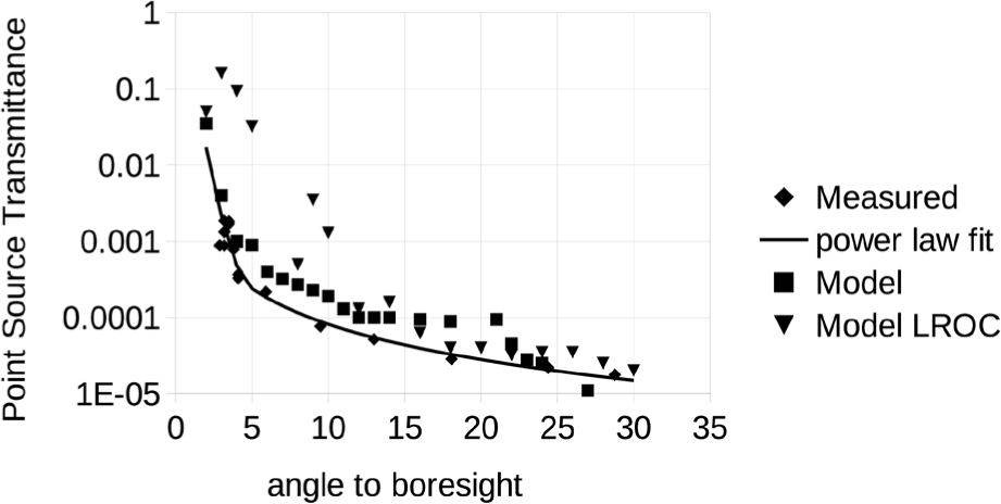
The measured PST values are a little lower than the modeled values but generally in good agreement. Fig. 28 also shows an empirical fit using the power law function PST = aθb with two different sets of parameters for two ranges. For θ between 2° and 4.5°, a = 0.604 and b = –5.144. For θ between 4.5° and 30°, a = 0.00292 and b = –1.55.
One can use this function to make rough estimates of out of field stray light background signal, given a large directly illuminated area nearby. For a stray light source which is dark everywhere, except for a spot outside the FOV covering the solid angle of a single ShadowCam pixel that has radiance Lsource, the formula for the equivalent stray light radiance Lstray is
Lstray is the radiance it would take to make the same signal the stray light makes. In keeping with the definition of PST, this is a mean value over the focal plane. PST(θ) is the PST as a function of the angle θ of the stray light source from the boresight. Apix = (12 × 10−6)2 is the area of one pixel on the focal plane in square meters. Aaper = π (0.194 / 2)2 is the area of the entrance pupil in square meters and η = 0.58 is the optical efficiency including the obscuration by the secondary mirror. Lsource is the radiance of the source, assumed to shine over the solid angle of just one ShadowCam pixel but outside the FOV.
For example, assuming a 1° square (1.03 million ShadowCam pixels) directly illuminated area 2° from the boresight (PST 0.0171) with radiance 5 W/m2/sr/µm, the resulting stray light equivalent radiance is 0.74 mW/m2/sr/µm, which is about 4 DN on the shallow side of the detector.
Fig. 29 illustrates detector artifacts and stray light that occur in ShadowCam images that have directly illuminated areas inside the FOV. The directly illuminated areas can have brightness more than 10 times the 4,095 DN saturation level of ShadowCam, so they are a strong source of stray light.
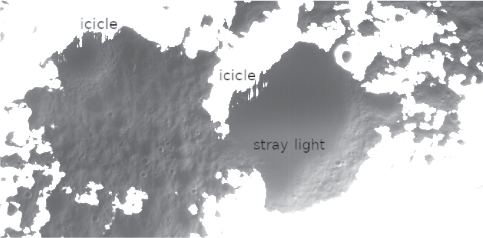
Fig. 29 is a selected area of image M012728826S, centered at sample 695, line 81,700. The image is fully calibrated except for the conversion to radiance. The stretch is 0–1,200 DN.
The “icicle artifact” is the most significant detector artifact. It can be seen at the boundary of the bright and dark areas at the top of the dark areas in Fig. 29. There are short bright stripes extending down from the saturated bright area, particularly evident in the upper left of the image. The icicle artifact always extends downtrack from the highly oversaturated area, never uptrack or crosstrack. Imaging is unaffected > 75 pixels from the directly illuminated area.
Stray light artifacts are much harder to identify in images than icicle artifacts. The stray light is quite diffuse so it will not be confused with small lunar features, but it can affect the measured radiance of the shadowed surface when that surface is within 150 pixels of a directly illuminated region.
The way to separate stray light in lunar images for the purpose of estimating its magnitude is to find an area of the image which has apparent signal but is devoid of small scale features. These areas do occasionally appear close to saturated areas of images. The interpretation is that this is actually a completely dark area, probably doubly shadowed, and all the signal is due to stray light.
One of these areas is evident in the upper central part of Fig. 29. It is a roughly circular area with icicle artifacts at the upper left. The upper part of this circular area is a little darker, with signal about 350 DN, and the lower part a little brighter, with signal about 540 DN. These are examples of high stray light DN levels for dark areas near highly oversaturated areas, as compared with stray light in other ShadowCam images. The interpretation is that the upper area is getting most of its stray light from above and the lower area from below, and the lower saturated area is clearly larger and may be brighter than the upper one. The lower area shows no icicle artifacts, but those artifacts only extend downward so we wouldn’t expect to see them there.
A different area of the same image, centered at sample 1,490 and line 10,475, is shown in Fig. 30 with stretch 0–400 DN. It gives a better idea of the geometry of this stray light. Again the image is fully calibrated except for the conversion to radiance.
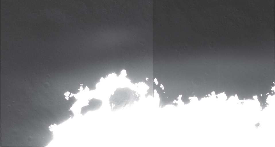
Note first the transition between the shallow side of the detector, which has higher gain, on the left, and the deep side of the detector with lower gain on the right. The gain difference is not of interest here but just applies a multiplier to the stray light.
One can see an area of stray light above the saturated area, but there’s clearly a boundary. In addition, on the shallow side at the top of the image there’s a separated stray light patch above the general area of stray light. In a fuzzy way this patch mirrors a separated saturated area above the main saturated area below it. This suggests that this stray light is more or less replicating the pattern of the source below but in a diffuse way.
The stray light peaks about 140 lines above the source. Unlike the previous example, the background isn’t perfectly featureless, but one can estimate the non-stray light signal from the darker area at the top of the image. The stray light is about 90 DN here in its brightest area on the upper part of the deep side.
We can check on this interpretation by looking at images of the Moon from cruise. Against the darkness of space there’s no question of these diffuse features being stray light and it’s possible to estimate the stray light signal as a fraction of the source.
Fig. 31 shows areas of CDRs E0097944719S through E007947719S of the nearly full Moon taken November 4, 2022 during the Earth to Moon cruise phase of the mission. These images are fully calibrated to radiance. The spacecraft traveled quite far from the Earth and Moon during cruise and the angular diameter of the Moon in these images is 3.4 times smaller than it is seen from the Earth. These images were captured with the Moon at different places in the FOV. For each image in Fig. 31, 463 samples by 477 lines are displayed, and the centers of the displayed area are (515,7600), (848,7655), (1178,7732), (1868,7695), (2217,7635), (2568,7560) for the 6 images. One can see the icicle artifact under each disk of the Moon. One can also see the stray light feature above and below the Moon. The stray light feature is clearly independent of position in the FOV.
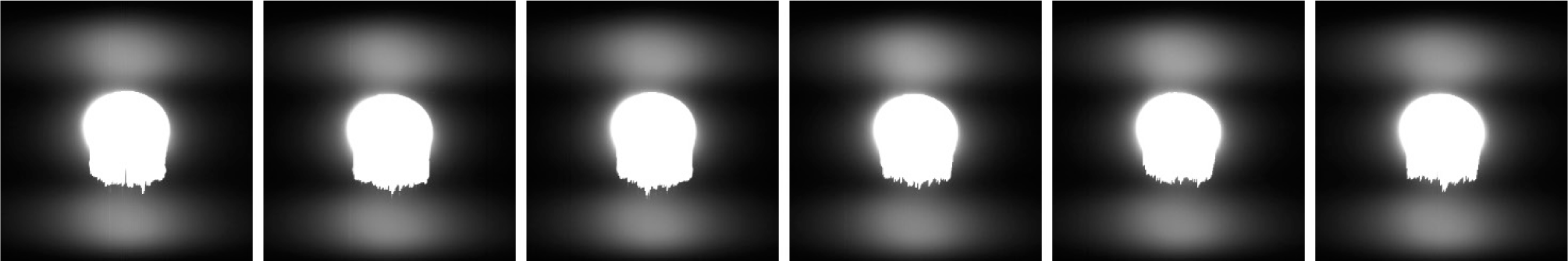
The peak of the stray light is approximately 140 lines above and 160 lines below the center of the lunar disk. The equivalent radiance to the stray light signal is approximately 0.12 W/m2/sr/µm at its peak. The full Moon is much brighter than directly illuminated lunar terrain near shadowed areas, due to both incidence angle and phase angle effects. The radiance of the full Moon over the ShadowCam bandpass is approximately 60 W/m2/sr/µm. So this stray light feature has equivalent radiance about 0.2% of the source in these cruise images.
The compact stray light source in these images shows the shape of the stray light feature well, but the fractional radiance should be smaller than one would see for a typical on-orbit image with stray light such as Figs. 29 and 30. The directly illuminated stray light source in Figs. 29 and 30 is a sizeable strip, not a small spot. In Fig. 31 the lateral extent of the stray light feature is larger than the source. If you had a horizontal strip the stray light would add up over a larger source solid angle and the fractional radiance would be larger. Earlier cruise images were taken with the angular size of the Moon only 1.4 times smaller than seen from Earth. That’s similar to the angular extent of the stray light feature. For those the stray light equivalent radiance peaks at about 0.5% of the source radiance and the peak occurs right at the limb of the Moon, both of which would be expected from the stray light pattern shown in Fig. 31.
The spatial location of the artifact in the cruise is in agreement with Figs. 29 and 30, but we can’t check the fractional radiance because we don’t know how bright the source regions are, just much brighter than the DN = 4,095 ShadowCam saturation level. To do a quantitiative check with ShadowCam images from lunar orbit we use a ShadowCam image with evident stray light for which there is an LROC image taken at a time of very similar subsolar point. We can use the LROC image to estimate the brightness of the directly illuminated area that is the source of the stray light.
Fig. 32 shows such an image pair. The ShadowCam CDR M017168767S (subsolar latitude -1.378°, longitude 189.547°) is shown on the left with a stretch 0–0.15 W/m2/sr/µm and LROC CDR M1102304370R (subsolar latitude –1.410°, longitude 189.515°) on the right with a stretch 0.07–0.22 W/m2/sr/µm. The stray light feature seen in Figs. 29–31 is also evident in the ShadowCam image at the top of the dark region in the center of the image, but it does not appear in the LROC image. The signal isn’t 100% stray light, as evident from a dim background with small craters, but the stray light component may be estimated by subtracting the mean radiance in the darker area below, and it’s about 0.04 W/m2/sr/µm. The LROC image measures radiance of 6.5 W/m2/sr/µm in the directly illuminated band right above that feature, the source of the stray light, which is saturated in the ShadowCam image. This indicates a stray light feature with radiance about 0.7% of the radiance of the source.
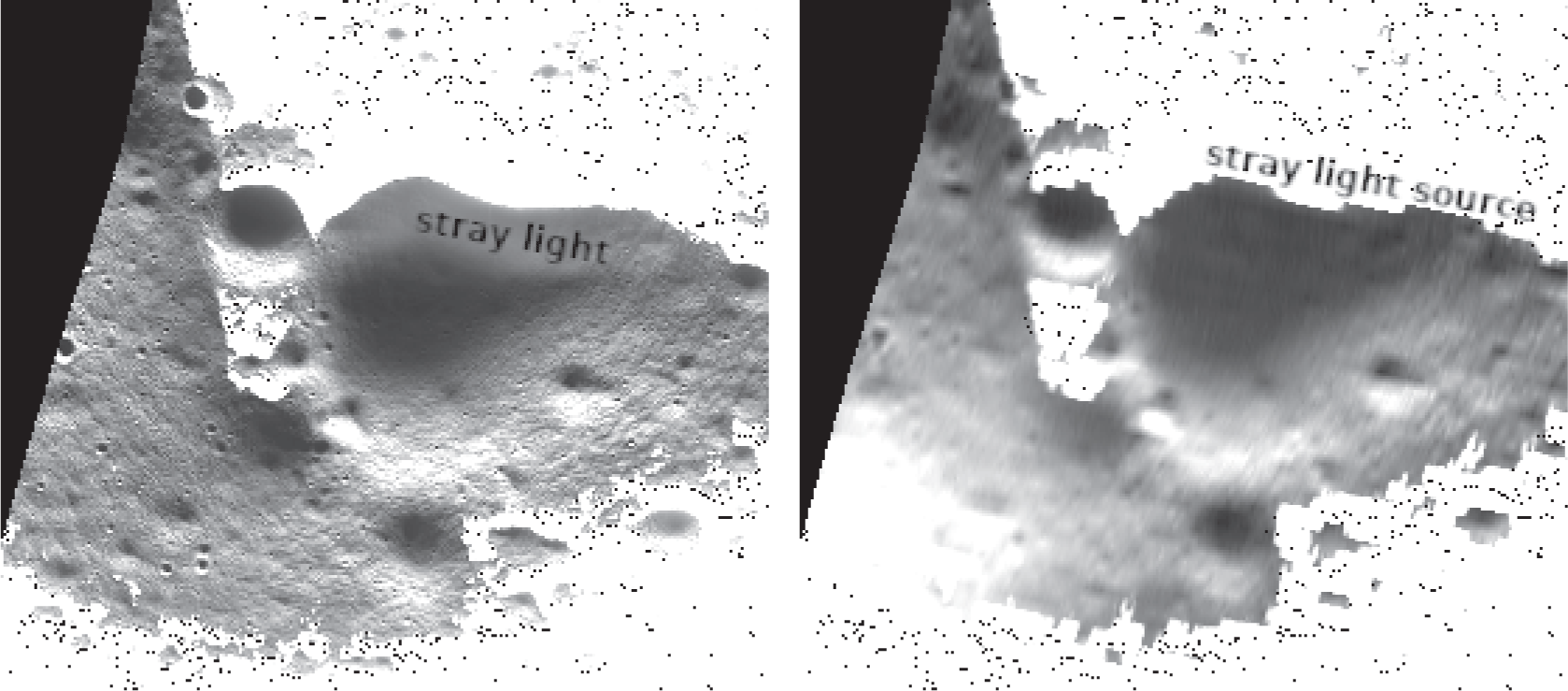
We calculated peak stray light effective radiance 0.2% of the source for a very compact source, 0.5% of the source for a source with greater angular extent, about the same as the stray light feature, and 0.7% for wide directly illuminated band on the lunar surface. This makes sense given the angular extent of the stray light feature. Because the stray light feature is limited in spatial extent, even larger stray light source areas will not increase the ratio much larger than 0.7%. Once the source area is much larger than the spatial extent of the feature, further increases would only spread the stray light to a wider area.
Fig. 33 shows the full width of 1,000 lines of the uncalibrated EDR M013110564S centered on line 46,900, displayed two ways, with stretch 25–50 at the top and 25–225 at the bottom. A slight dark pattern is seen repeated in channels 0, 1, 2, and 3 of the top image. It approximately replicates the shape of the bright pattern seen in channel 4 of the bottom image, which is the source of the crosstalk. The cruise images of the Moon showed that this crosstalk occurs in the other channels when there is a bright area in channel 3 or 4. The crosstalk is not a simple function of the brightness of the source, so it is not practical to implement a correction. However, the amplitude after decompanding is only 6 DN at most, so it is not very important. In fact it is difficult to find an image where it is visible.
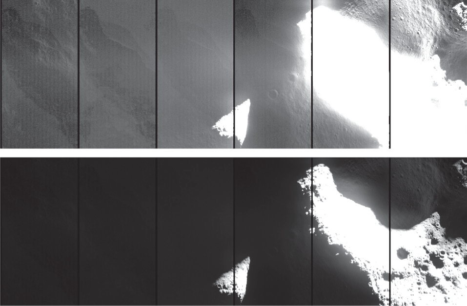
The icicle and stray light artifacts discussed in the previous section are by far the most important artifacts in science images. There are other diffuse stray light artifacts in the science images but, like the channel crosstalk, they contribute only a few DN to the signal.
ShadowCam is a nadir viewing instrument, so when it is on the night side and the KPLO spacecraft is not yet in the Moon’s shadow, the Sun is in the front and shines inside the sunshade. This results in a stray light artifact consisting of broad vertical stripes in dark calibration images taken on the night side, as shown in Fig. 34. The top image M21139099S, taken at Sun-boresight angle 97.895°, has the baseline pattern that is fairly constant and shows up at all angles from 95-110°. The bottom image M20842357S, taken at Sun-boresight angle 104.046° is a fairly severe example of the brighter bar that shows up on the right side from 103°–110°.
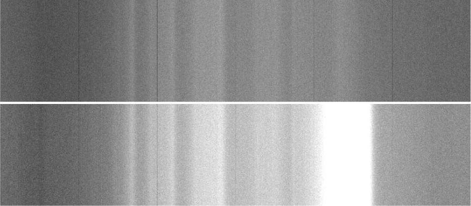
Fig. 35 shows the equivalent radiance (95th percentile value for each image) of this stray light feature as a function of phase angle. This stray light feature is very evident since it shows up in calibration images taken to monitor the dark level. It is not important for science images. For phase angle < 90° the Sun does not shine into the front of the sunshade and this feature does not occur.
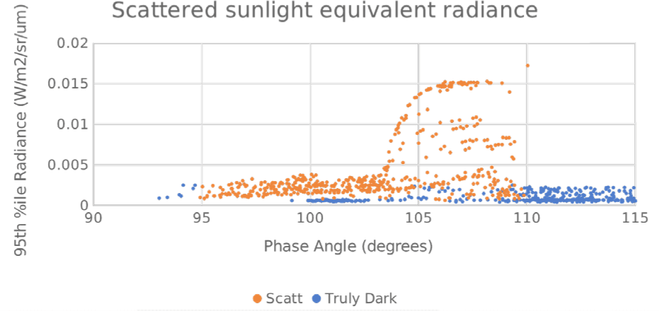
8. CONCLUSION
ShadowCam performance meets the requirements of an instrument to fully image lunar PSRs with 1.7 meter/pixel image scale, a data set heretofore not available. The radiometric accuracy is conservatively estimated at 6%, and the responsivity is high enough to image the vast majority of lunar PSR pixels. In some cases ShadowCam can even image the night side using Earthshine (Wagner et al. 2023). The SNR is > 100 over a large part of the dynamic range, and the top of the dynamic range is high enough to accommodate most brighter PSR pixels.
ShadowCam image quality is good. System MTF is high enough to give good resolution at the pixel scale, similar to the LROC NAC from which the optical design was derived. Dark subtraction is accurate, and the calibrated images have uniform response down to the noise level except for a few columns, particularly the first column of each channel.
Stray light control is challenging for a sensitive instrument like ShadowCam that images very dark areas which can sometimes be close to fully illuminated terrain. The modifications to the LROC NAC design for stray light control were successful. In many cases imaging is possible with fully illuminated terrain in or near the FOV. We have presented a thorough qualitative description of the circumstances under which lunar brightness levels far higher than the top of the dynamic range can cause detector artifacts or evident stray light, and the size and extent of the artifact or stray light signal under those circumstances.
Some remaining image artifacts are amenable to correction. They result from a small discrepency in timing between the detector and electronics. They include the striping and pepper noise that appear at large signal level and affect image uniformity, and the column transfer of signal, which also gets worse at large signal level and reduces MTF. If corrections are implemented for these artifacts the imaging will be further improved, particularly for brighter areas of the PSRs.